How to Use Conditional Formatting in Excel: The Complete Guide

Have you ever stared at a spreadsheet filled with thousands of numbers, trying to spot the trends? It is exhausting. Finding the lowest sales figure or the students who failed an exam shouldn’t involve squinting at rows for hours.

You need Conditional Formatting.

This feature allows Excel to automatically change the color, font, or border of a cell based on its value. Think of it as a “live highlighter” that reacts to your data. If a number goes down, it turns red. If it goes up, it turns green.

In this ultimate guide, we will cover everything from basic color scales to advanced formulas that highlight entire rows.

What is Conditional Formatting?

Conditional Formatting commands Excel to apply a specific style only when a specific condition is met.

Common uses:

• Highlighting duplicates.
• Identifying tasks that are “Overdue”.
• Visualizing data distribution with heat maps.
• Creating progress bars inside cells.

Level 1: Highlighting Cells Rules (The Basics)

Let’s say you want to highlight any test score below 50 in Red.

1. Select your data: Highlight the column with the scores (e.g., the Math Score column).
2. Go to Home Tab: Click on Conditional Formatting in the Styles group.

1. Hover over Highlight Cells Rules: Select Less Than…
2. Set the Rule:
   • In the box, type 50.
   • In the dropdown next to it, select Light Red Fill with Dark Red Text.

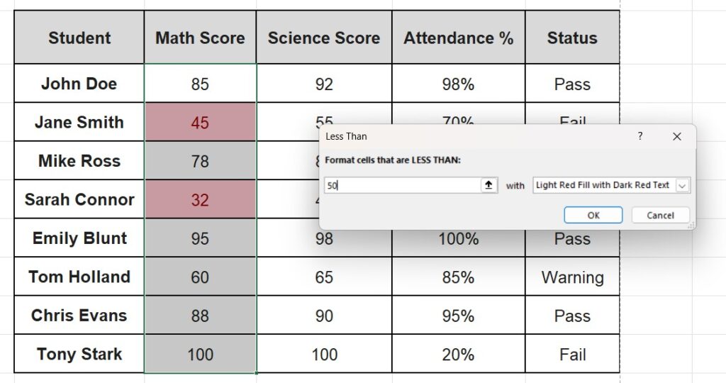
1. Click OK.

Instantly, all failing grades are highlighted. If you change a score from 45 to 80, the red highlight disappears automatically.

Level 2: Data Bars and Color Scales (Visualizing Density)

You can turn your cells into mini-charts without inserting a graph.

Data Bars (Progress Bars)

This is perfect for “Attendance %” or “Sales Targets”.

1. Select the Attendance column.
2. Go to Conditional Formatting > Data Bars.
3. Pick a color (e.g., Blue Data Bar).

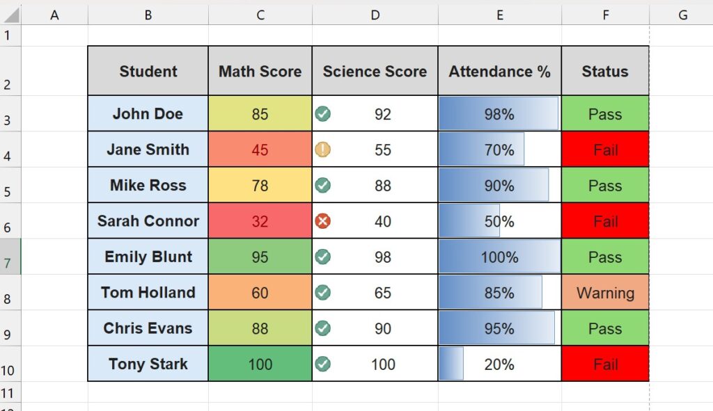
Excel fills the cell with a blue bar proportional to the number. 100% fills the cell; 50% fills half. It is the fastest way to compare numbers visually.

Color Scales (Heat Maps)

This creates a “thermal map” where high numbers are green and low numbers are red.

1. Select your numerical data.
2. Go to Conditional Formatting > Color Scales.
3. Pick the first option (Green – Yellow – Red).

Now you can spot the highest and lowest performers in milliseconds.

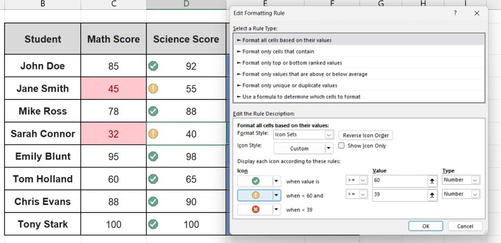
Level 3: Icon Sets (Traffic Lights)

Managers love this one. You can add arrows, flags, or traffic lights to your data.

1. Select your data (e.g., Science Score).
2. Go to Conditional Formatting > Icon Sets.
3. Choose the Shapes (Traffic lights) or Indicators (Checkmarks/X).

Pro Tip: By default, Excel calculates the split based on percentiles (top 33% gets green). To customize this, go to Manage Rules > Edit Rule and change the Types to “Number” to set your own passing thresholds.

Level 4: Highlight Entire Rows Based on One Cell (Advanced)

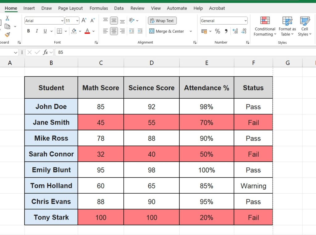
This is the “Holy Grail” of conditional formatting. Instead of just coloring the cell that says “Fail”, you want to color the entire row for that student red.

The built-in buttons won’t do this. You need a formula.

Step 1: Select the Whole Dataset Highlight your entire table (excluding headers). e.g., C3:F10.

Step 2: Create a New Rule Go to Conditional Formatting > New Rule.

Step 3: Use a Formula Select the last option: “Use a formula to determine which cells to format”.

Step 4: Write the Formula We want to check if the “Status” column (Column E) says “Fail”. Type this formula: =$F3="Fail"

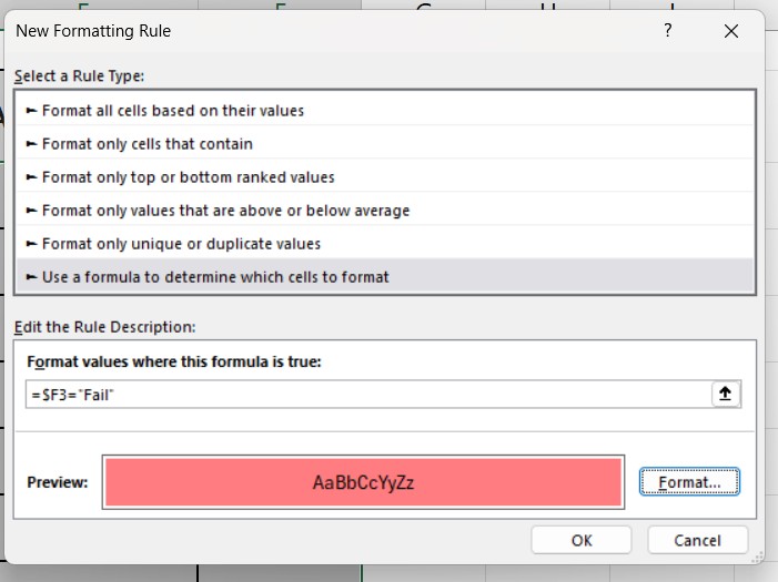
• Important: Notice the $ sign before the F ($F), but NOT before the 3. This “locks” the column so Excel always checks column E, but lets the row number change as it goes down the list.

Step 5: Set the Format Click the Format button. Go to the Fill tab and choose a light red background. Click OK twice.

Now, any student with “Fail” status has their whole row highlighted.

How to Manage and Delete Rules

Did you make a mess? Don’t worry.

• To Clear: Go to Conditional Formatting > Clear Rules > Clear Rules from Selected Cells.
• To Edit: Go to Conditional Formatting > Manage Rules. Here you can see all active rules, change their order, or edit their logic.

Frequently Asked Questions (FAQ)

Does Conditional Formatting make Excel slow? Generally, no. However, if you apply thousands of complex formula-based rules to a massive dataset, it can slow down calculation speed. Use it wisely.

Can I use Conditional Formatting based on another sheet? Yes, but only in newer versions of Excel. In older versions, you might need to use the INDIRECT function to reference other sheets within a conditional formatting rule.

Combine this with Drop-Downs Conditional formatting works amazingly well with interactive lists. Learn How to Create a Drop-Down List in Excel and then use formatting to color-code your choices (Green for “Yes”, Red for “No”)