How to Unhide All Rows in Excel: The Ultimate Guide (Shortcuts & Fixes)

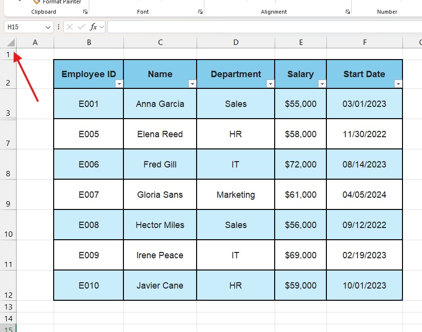
We have all been there. You open a spreadsheet sent by a colleague, and the row numbers jump from 5 to 50. Data is missing. You try to right-click and “Unhide,” but nothing happens. Frustrating, right?

Learning how to unhide all rows in Excel sounds simple, but it is often trickier than it looks. Sometimes rows are hidden manually, sometimes they are trapped behind a filter, and sometimes they are “shrunk” to zero height.

In this comprehensive guide, we will cover every single method to reveal your data—from the fastest keyboard shortcuts to advanced troubleshooting techniques for when the buttons just won’t work.

Method 1: The “Select All” Trick (Best for Beginners)

If you want to unhide absolutely everything on your sheet in one go, this is the most reliable method. It ensures you don’t miss any hidden sections. This is often the quickest solution when learning how to unhide all rows in Excel for the first time.

Step-by-Step:

1. Select the Entire Sheet: Click the small triangle icon in the top-left corner of the grid (exactly where the row numbers and column letters meet).
   • Alternative: Press Ctrl + A (you might need to press it twice to select the whole sheet).

1. Right-Click: Move your mouse over any row number (e.g., row 5). It is important to click on the number itself, not inside the grid.
2. Choose Unhide: Select Unhide from the context menu.

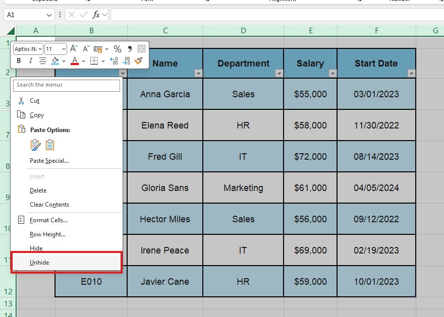
Boom. Every hidden row in your entire spreadsheet should reappear instantly.

Method 2: The Keyboard Shortcut (The “Pro” Way)

Stop using the mouse. If you want to impress your boss or simply work faster, you need to master the shortcut for how to unhide all rows in Excel.

The Magic Combination:

• Windows: Ctrl + Shift + 9 (Note: Use the 9 on the top row of your keyboard, not the number pad).
• Mac: Command + Shift + 9

How to use it:

1. Select the rows surrounding the hidden section (or press Ctrl + A to select all).
2. Hit Ctrl + Shift + 9.
3. The hidden rows will expand immediately.

Memorization Tip: Why 9? Because Ctrl + 9 hides rows. Adding Shift reverses the action.

Method 3: The “Double-Click” Technique

Sometimes you don’t want to unhide all rows, but just a specific section without selecting huge ranges.

1. Look at the row numbers on the left.
2. Find the gap (e.g., it goes from row 10 to row 15).
3. Hover your mouse cursor exactly over the line between the number 10 and 15 headers.
4. Your cursor will change into a double bar with two arrows (up and down).
5. Double-click quickly.

This instantly reveals the hidden rows between those two points. It is precise and fast.

Troubleshooting: “Why Can’t I Unhide Rows in Excel?”

This is the part that drives people crazy. You followed the steps above on how to unhide all rows in Excel, but the rows are still missing.

If “Unhide” isn’t working, you are likely facing one of these three common traps.

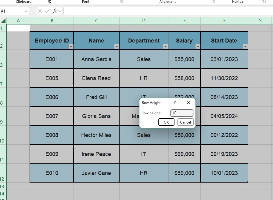
Trap A: The “Row Height” Bug

Sometimes rows aren’t technically “hidden”; they just have a height of 0.1 or 0. Excel treats them as visible, so the “Unhide” button does nothing.

The Fix:

1. Select the entire sheet (Ctrl + A).
2. Right-click on any row number.
3. Select Row Height…
4. Type a standard value like 15 or 20.
5. Click OK. Your rows will pop open because you forced them to have a visible size.

Trap B: The “Filter” Trap

If your row numbers are blue instead of black, your rows aren’t hidden—they are filtered out. The “Unhide” command does not work on filters.

The Fix:

1. Go to the Data tab on the ribbon.
2. Look for the Clear button (next to the big Filter icon).
3. Click it to clear all active filters.
4. Alternatively, press Ctrl + Shift + L to toggle filters off completely.

Trap C: Frozen Panes Confusion

Sometimes rows 1 to 10 seem “gone,” but they are actually just scrolled out of view because of “Freeze Panes.”

The Fix:

1. Go to the View tab.
2. Click Freeze Panes.
3. Select Unfreeze Panes.
4. Scroll up to the top of your sheet.

Pro Tip: Managing large datasets can be tricky. If you often lose sight of your headers while scrolling through your newly unhidden rows, we highly recommend you read our guide on How to Freeze the Top Row in Excel.

Advanced: Using “Go To Special” for Visible Cells

If you are copying data and only want to copy the rows you can see (ignoring the hidden ones), beginners often make a mistake. They copy/paste and accidentally bring the hidden data with them.

How to select ONLY visible rows:

1. Select your dataset.
2. Press F5 on your keyboard (Go To).
3. Click Special…
4. Choose Visible cells only.
5. Click OK.
6. Now copy (Ctrl + C) and paste.

Shortcut: Alt + ; (Semicolon) selects visible cells instantly.

Frequently Asked Questions (FAQ)

Is there a VBA code to unhide all rows? Yes. If you have a massive workbook with multiple sheets and want to unhide everything at once, use this simple macro: Sub UnhideAllRows() Rows.EntireRow.Hidden = False End Sub

Does deleting rows make them unrecoverable? Yes. “Hiding” is temporary; “Deleting” is permanent. If you accidentally deleted rows instead of hiding them, press Ctrl + Z (Undo) immediately. If you saved and closed the file, the data is gone unless you have a backup version.

Why are my row numbers missing entirely? If you don’t see any row numbers on the left, you might have hidden the Headings. Go to View > Show and ensure the Headings box is checked.

Conclusion

Mastering how to unhide all rows in Excel is a fundamental skill for data hygiene. Whether it is a simple right-click, a “ninja” keyboard shortcut, or fixing a zero-height glitch, you now have the toolkit to ensure no data ever stays lost in your spreadsheets.

Next time you receive a confusing file with missing numbers, you will know exactly which trick to use.