How to Sort Columns in Excel: The Ultimate Guide to Sorting Left to Right (2025)

Learning how to sort columns in Excel is a game-changer when dealing with horizontal datasets. Most Excel users know how to sort rows (top to bottom), but they get stuck when data is messy horizontally (left to right). In this guide, we will show you exactly how to do it.

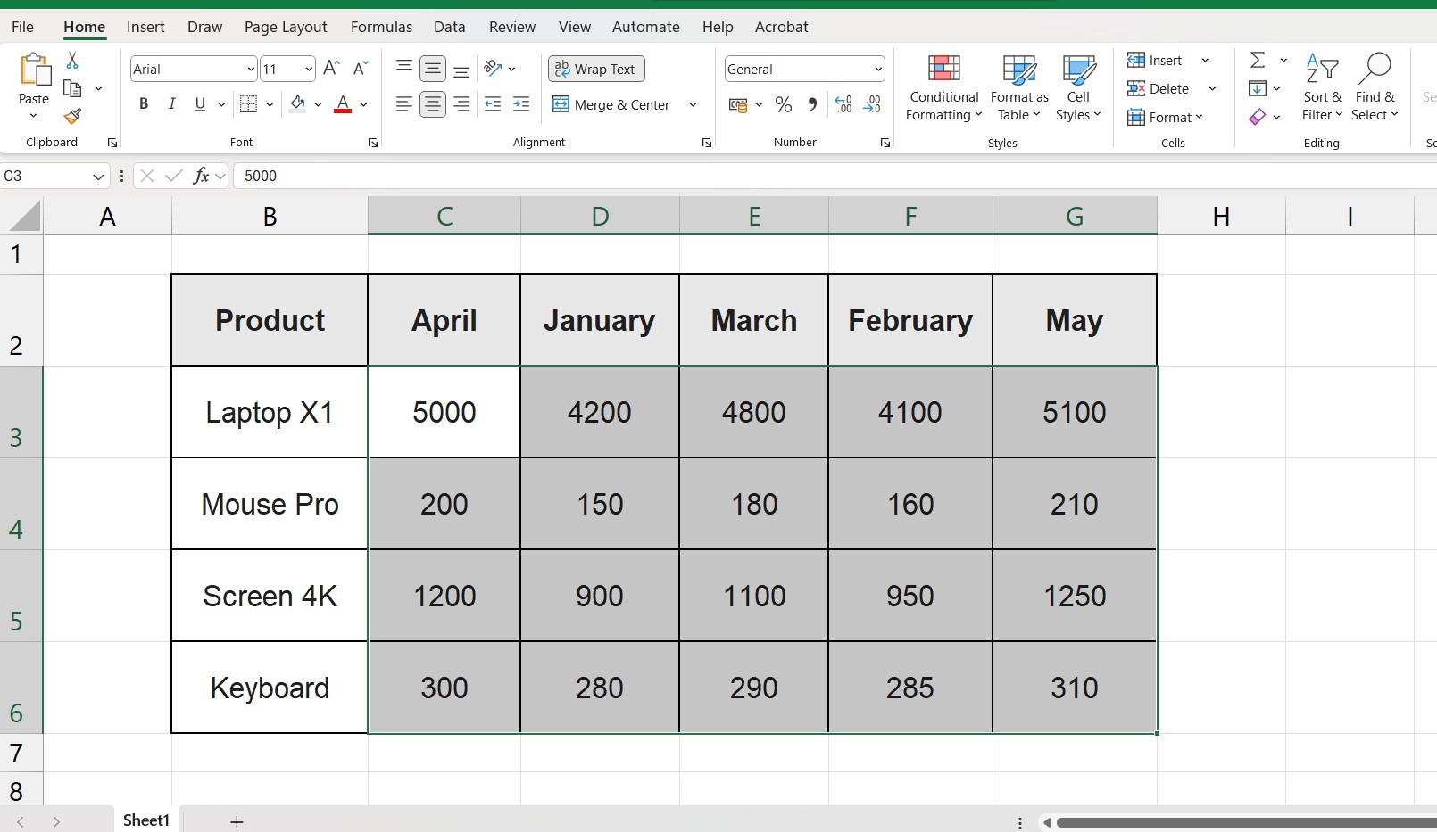
Imagine you have a report where the months are out of order (e.g., March, January, April, February) across the top row, or you have a dataset with 50 columns that need to be alphabetized by their headers. Dragging and dropping columns one by one is slow and prone to errors.

There is a better way.

In this guide, you will learn how to sort columns in Excel (sorting from left to right). We will cover the hidden “Sort Options” feature that 90% of users miss, and how to use dynamic formulas for modern sorting.

Why Can’t I Just Use the Filter Button?

By default, Excel assumes your data is organized in lists (vertical). When you click the standard “Sort & Filter” buttons, Excel looks for rows to reorganize. To sort columns, we need to change Excel’s orientation setting in the Custom Sort menu.

Here are the 3 best methods to sort your columns instantly.

---

Method 1: How to Sort Columns in Excel Alphabetically

This is the most compatible method and works in every version of Excel. We will tell Excel to sort “Left to Right” instead of “Top to Bottom.”

Step 1: Select Your Data Range

Select the columns you want to sort.

• Important: Do not select the “Row Labels” column (usually Column A) if you want that to stay fixed on the left. Only select the data columns that need moving.

Step 2: Open the Custom Sort Dialog

1. Go to the Data tab on the Ribbon.
2. Click on Sort (not the small A-Z icons, but the larger Sort button).

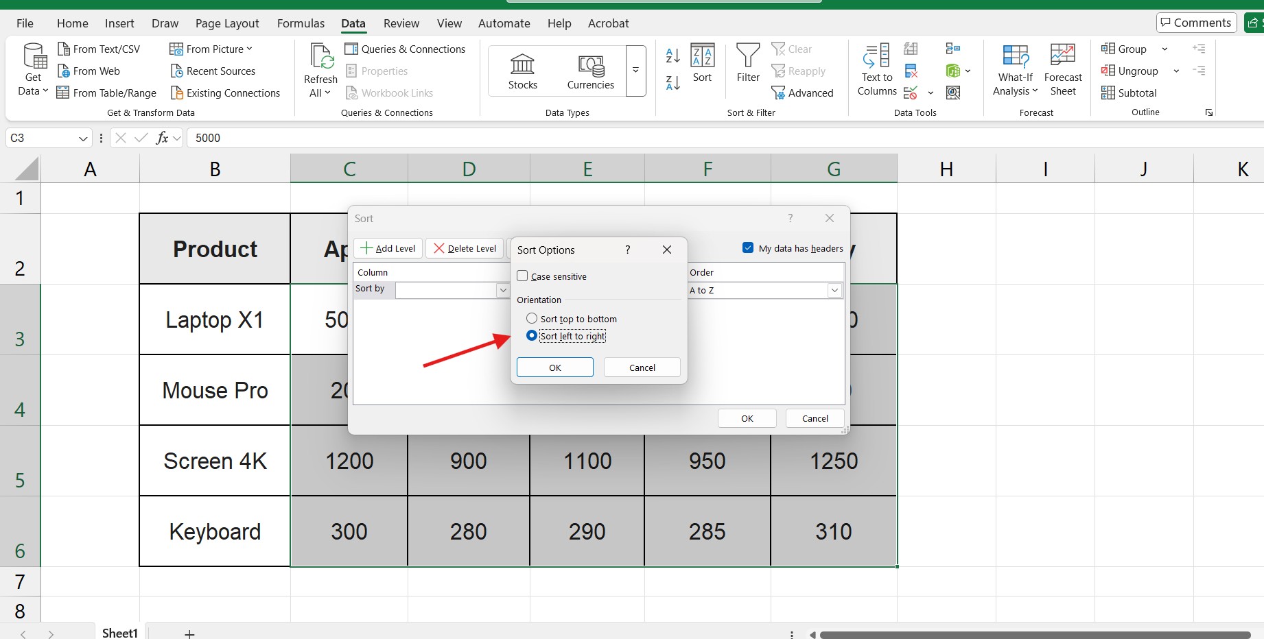
Step 3: Change Orientation to “Left to Right”

This is the secret step.

1. Inside the Sort dialog box, click the Options… button at the top.
2. A small window will pop up. Select Sort left to right.
3. Click OK.

Step 4: Choose Your Sort Criteria

Now that Excel knows you are sorting horizontally:

1. In the “Sort by” dropdown, select Row 1 (or whichever row contains your headers/titles).
2. Ensure “Order” is set to A to Z.
3. Click OK.

Your columns will instantly rearrange themselves alphabetically!

Method 2: Sort Columns by Month or Custom List

Knowing how to sort columns in Excel alphabetically is great, but sometimes you need chronological order (like months or days). Sorting alphabetically isn’t always helpful. If you sort months alphabetically, you get April, August, December… which is useless for a timeline. You need to sort chronologically (Jan, Feb, Mar).

1. Select your data range (again, exclude the fixed label column).
2. Go to Data > Sort.
3. Click Options… and ensure Sort left to right is selected.
4. In the “Order” dropdown, instead of A to Z, select Custom List…
5. Choose the list that matches your data (e.g., Jan, Feb, Mar or Sunday, Monday, Tuesday).
6. Click OK.

Excel will now reorder your columns based on the calendar logic, not the alphabet.

Method 3: Using the SORT Function (Excel 365 & 2021)

If you have a modern version of Excel, you can use a formula to create a sorted copy of your data. This is dynamic—if you change a header name, the sorted list updates automatically.

We use the =SORT function, specifically the 4th argument which controls the direction. You can read the official documentation on the Microsoft Support SORT function page for more technical details.

The Formula: =SORT(array, sort_index, sort_order, by_col)

• array: The range you want to sort (e.g., B1:G10).
• sort_index: The row number to sort by (usually 1 for the header).
• sort_order: 1 for ascending, -1 for descending.
• by_col: Set this to TRUE to sort horizontally.

Example: To sort the range B1:G10 based on the headers in the first row: =SORT(B1:G10, 1, 1, TRUE)

Note: This creates a “Spill” range. Make sure you have empty space to the right of your formula. If you see an error, check our guide on the SPILL! Error in Excel.

Pro Tip: Sorting Columns to Match Another Table

Sometimes you don’t need A-Z or Jan-Dec sorting. You might need your columns to match a specific order from a different report (e.g., Revenue, Cost, Profit, Tax).

To do this:

1. Create a Custom List with those exact headers (File > Options > Advanced > Edit Custom Lists).
2. Use Method 2 above and select your new custom list.

This is a massive time-saver for financial analysts who need to standardize multiple reports.

---

FAQ: Troubleshooting Column Sorting

Q: Why is the “Sort” button grayed out? A: This usually happens if you have grouped sheets (multiple tabs selected at once) or if you are in “Edit Mode” inside a cell. Press Esc and try again. Also, ensure your sheet isn’t protected. If it is, you might need to check How to Lock Cells in Excel to understand permissions.

Q: Can I restore the original order after sorting? A: If you just did it, use Ctrl + Z. If you saved the file, you cannot “unsort” unless you have a helper row numbered 1, 2, 3… that represents the original order. It is always best to Make a Copy of Your Excel Sheet before doing major data restructuring.

Q: Does this move the data below the headers? A: Yes! When you use “Sort Left to Right”, Excel moves the entire column (the header and all data below it) together. Your data integrity remains safe.

---

Summary

Mastering how to sort columns in Excel will save you hours of manual copy-pasting.

1. Data > Sort.
2. Options > Sort left to right.
3. Select the Row you want to sort by.

Now that your columns are organized, you might want to format them for better readability. Check out our guide on How to Alternate Row Colors to make your new layout pop!