How to Freeze the Top Row in Excel (Keep Headers Visible While Scrolling)

We have all been there. You are looking at a massive spreadsheet with thousands of rows. You scroll down to row 500 to check a specific value, but suddenly, you realize you have no idea what column you are looking at.

“Is this number the Sales Price or the Cost Price? Is this date the Order Date or the Ship Date?”

To find out, you have to scroll all the way back up to the top, check the header, and scroll back down. It is frustrating and wastes time.

The solution is to Freeze Panes.

In this guide, you will learn how to lock rows and columns in Excel so that your headers remain visible no matter how far you scroll.

Method 1: Freezing the Top Row (The Most Common Fix)

If you just want to keep your headers (Row 1) visible, Excel has a dedicated button for this. It takes literally two clicks.

1. Open your Excel worksheet.
2. Go to the View tab on the top ribbon.
3. Look for the “Window” group and click on Freeze Panes.

1. Select the second option: Freeze Top Row.

How do you know it worked? You will see a thin, solid line appear under Row 1. Now, try scrolling down. Row 1 will stick to the top of your screen while the rest of the data moves.

Method 2: Freezing the First Column

Sometimes, your dataset is very wide (many columns), and you lose track of the names on the left as you scroll to the right.

1. Go to the View tab.
2. Click on Freeze Panes.
3. Select the third option: Freeze First Column.

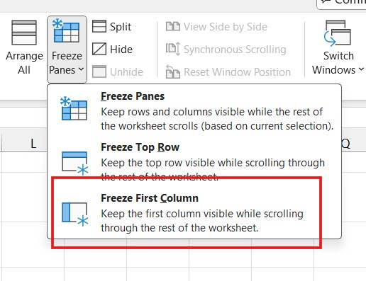
Now, Column A will remain locked in place as you scroll horizontally.

Method 3: Freezing Multiple Rows or Columns (The “Magic Cell” Trick)

This is where most beginners get stuck. What if your headers take up the first three rows? Or what if you want to lock the top row AND the first two columns at the same time?

The built-in buttons (“Freeze Top Row”) won’t work here. You need to use the custom Freeze Panes option. The trick is selecting the correct cell before you click the button.

The Rule of the “Magic Cell”: Excel will always freeze everything above and to the left of the cell you select.

Example A: Freezing the Top 3 Rows

If you want Rows 1, 2, and 3 to stay fixed:

1. Click on cell A4 (Because A4 is just below Row 3).
2. Go to View > Freeze Panes.
3. Click the first option: Freeze Panes.

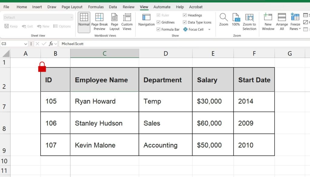
Example B: Freezing Row 1 and Column A (Both)

If you want to lock the header at the top and the names on the left:

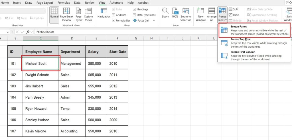
1. Click on cell C3.
   • Why C3? Because it is just below Row 1 and just to the right of Column A.
2. Go to View > Freeze Panes > Freeze Panes.

Now you have a professional dashboard that is easy to navigate in any direction.

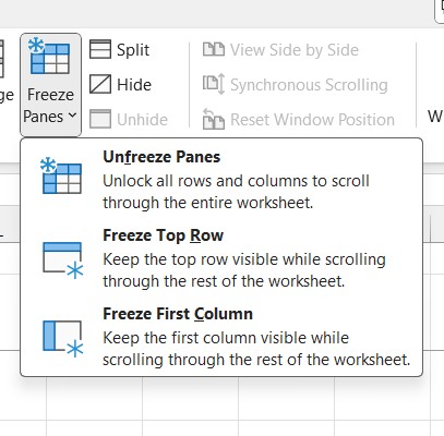
How to Unfreeze Panes

If you made a mistake or just want to return the sheet to normal:

1. Go to the View tab.
2. Click on Freeze Panes.
3. Select Unfreeze Panes.
   • Note: This option only appears if you already have something frozen.

Troubleshooting: Why is “Freeze Panes” Grayed Out?

Sometimes you might go to the View tab and find that the Freeze Panes button is gray and unclickable. This usually happens for one reason: Page Layout View.

Excel cannot freeze panes while you are in “Page Layout” mode (the view used for printing setup).

The Fix:

1. Go to the View tab.
2. On the far left, click on Normal (Workbook Views).
3. The Freeze Panes button should now be active again.

Frequently Asked Questions (FAQ)

Does freezing rows affect printing? No. Freezing panes only affects what you see on the screen. If you want your headers to appear on every page when you print, you need a different feature called “Print Titles” (found in the Page Layout tab).

Can I freeze rows in the middle of the sheet? No, Excel only allows you to freeze rows starting from the top or columns starting from the left. You cannot freeze “Row 10” while letting Rows 1-9 scroll.

Organizing your data? Now that your view is set up, make sure your data entry is clean. Check out our guide on How to Create a Drop-Down List in Excel.