
You have a spreadsheet with “First Name” in Column A and “Last Name” in Column B. Your boss asks for a single “Full Name” column.
Do you retype hundreds of names manually? Absolutely not.
Learning how to combine two columns in Excel is one of the most essential skills for data analysis. Whether you are merging names, creating addresses, or generating unique IDs, you need to know how to join text efficiently.
Unlike “Merging Cells” (which destroys data), combining text creates a new, clean text string without losing anything.
In this comprehensive guide, we will explore 5 proven methods to merge columns in Excel. We will cover everything from the classic Ampersand (&) symbol to the modern TEXTJOIN function and the “no-formula” magic of Flash Fill.
We will also solve the #1 problem users face: How to combine two columns in excel, text with dates or numbers without losing the formatting.
Method 1: The Ampersand (&) Symbol (The Fastest Way)
The & symbol is the “glue” of Excel. It allows you to stick different pieces of text together instantly. It is faster than typing a function name and works in every version of Excel.
The Scenario: You want to combine “John” (Cell B3) and “Doe” (Cell C3).
The Common Mistake: If you simply type =B3&C3, Excel will give you JohnDoe (no space). This looks unprofessional.
The Solution: You must manually “glue” a space in the middle using double quotes.
Formula:
=B3 & " " & C3- Breakdown: Join Content of B3 + a Space (inside quotes) + Content of C3.
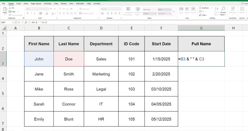
This method is the fastest way to combine two columns in Excel if you only have a small dataset. You can use it to add commas too: =B3 & ", " & C3.
Method 2: The CONCAT Function (The Modern Standard)
For years, people used CONCATENATE (a long, hard-to-spell word). Microsoft has replaced it with the newer, shorter CONCAT function (available in Excel 2019 and Office 365).
It works similarly to the & symbol but is easier to read if you are joining many cells or ranges.
Formula:
=CONCAT(A2, " ", B2)Note: If you are using an older version of Excel (Excel 2016 or older), you may still need to use =CONCATENATE(). Both work, but CONCAT is preferred for modern workflows.
Method 3: TEXTJOIN (The “Game Changer” for Lists)
What if you need to combine 10 columns (e.g., First Name, Last Name, Email, Dept, City…) and you want a comma between each one?
Typing A2 & ", " & B2 & ", " & C2... takes forever and is prone to errors.
Enter TEXTJOIN. This powerful function allows you to specify a “delimiter” (separator) once, and Excel applies it to everything automatically.
Syntax: =TEXTJOIN(delimiter, ignore_empty, range)
Example: Creating a comma-separated list
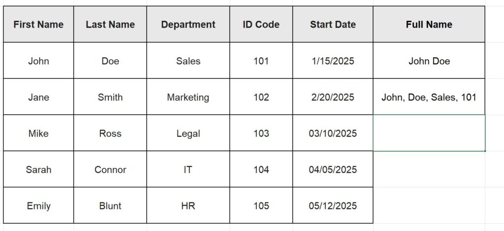
=TEXTJOIN(", ", TRUE, B3:E3)- “, “: The separator (comma and space).
- TRUE: Tells Excel to ignore blank cells (so you don’t get double commas like “Apple,, Banana”).
- B3:E3: The range of cells to combine.

Result: John, Doe, Sales, 101
Method 4: Flash Fill (No Formulas Required)
This is the user-favorite method because it requires zero code. It uses Artificial Intelligence to guess what you want to do.
How to do it:
- Type the full result you want in the first cell (e.g., manually type “John Doe – Sales”).
- Click the cell below it.
- Press Ctrl + E.
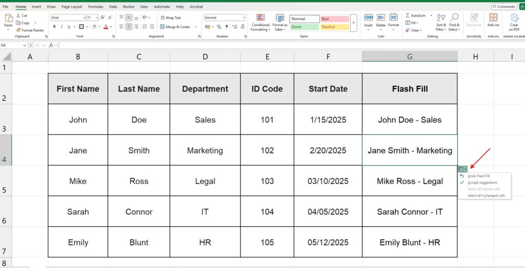
Excel detects that you are combining Column A, Column B, and Column C with a hyphen, and applies that pattern to the next 1,000 rows instantly.
Warning: Flash Fill is static. If you change “John” to “Jonathan” in column A, the combined cell will NOT update automatically. Use formulas if you need dynamic data.
Method 5: Power Query (For Professional Data Shaping)
If you are cleaning a massive dataset (100,000+ rows) for a dashboard, formulas might slow down your computer. Power Query is the professional solution.
- Select your data and go to Data > From Table/Range.
- In the Power Query Editor, hold Ctrl and click the columns you want to combine (e.g., First Name and Last Name).
- Right-click on one of the headers.
- Select Merge Columns.
- Choose your separator (Space, Comma, Custom).
- Click OK and then Close & Load.
This creates a robust process that you can refresh anytime new data arrives.
Common Problem: Combining Text and Dates
This is where 90% of users get stuck. They try to combine two columns in Excel with text and dates.
Imagine you want to create a sentence: “John joined on 1/15/2025”.
If you type =A2 & " joined on " & E2, Excel will return: “John joined on 45672”
Why? Because Excel stores dates as serial numbers. When you combine them with text, the visual formatting is lost.
The Fix: The TEXT Function You must tell Excel how to read the date inside the formula using the TEXT function.
Correct Formula:
=A2 & " joined on " & TEXT(E2, "mm/dd/yyyy")This forces the number 45672 to display as “01/15/2025”. You can change the format to “dd-mmm-yy” (15-Jan-25) or whatever you prefer.

Advanced Tip: Adding Line Breaks in Formulas
Want to combine an address so it appears on multiple lines inside one cell?
- Street
- City
- Zip
You need the CHAR(10) code, which represents a “Line Break” in Windows.
Formula: =A2 & CHAR(10) & B2 & CHAR(10) & C2
Crucial Step: After pressing Enter, you must click Wrap Text on the Home tab to see the lines break correctly.
Frequently Asked Questions (FAQ)
What is the difference when you combine two columns in Excel vs Merging?
- Merging Cells (the button in the ribbon) combines the space of two cells into one big cell, but it deletes the data in the second cell (keeping only the top-left value).
- Combining Cells (using formulas like
&orCONCAT) keeps all the data and joins it into a new text string. Always combine, never merge data if you want to keep the information.
Can I combine two columns in Excel with formatting (e.g., Bold part of it)? No. Excel formulas return plain text. You cannot have the first word Bold and the second word Italic inside a formula result. To do that, you would need to Copy > Paste Values and then format the text manually or use a VBA script.
How do I separate them back? If you combined data by mistake or received a combined file, you can reverse this process. Check out our guide on How to Split Text to Columns in Excel.
Analyze your new data Now that your columns are combined and clean, you are ready for analysis. Learn how to summarize your data with our guide on How to Create a Pivot Table in Excel.