How to Alternate Row Colors in Excel (The “Zebra Stripe” Guide)

Reading a spreadsheet with hundreds of rows can be a headache. Your eyes naturally jump from one line to another, leading to mistakes.

The solution? Alternating Row Colors (often called “Zebra Stripes”).

By shading every other row, you make your data instantly readable and professional.

In this guide, you will learn the 2 fastest ways to do this: the “One-Click” method (Table Format) and the “Pro” method (Conditional Formatting).

Method 1: Format as Table (The Fastest Way)

This is the easiest method and takes literally two clicks.

1. Select your entire dataset.
2. Go to the Home tab on the top ribbon.
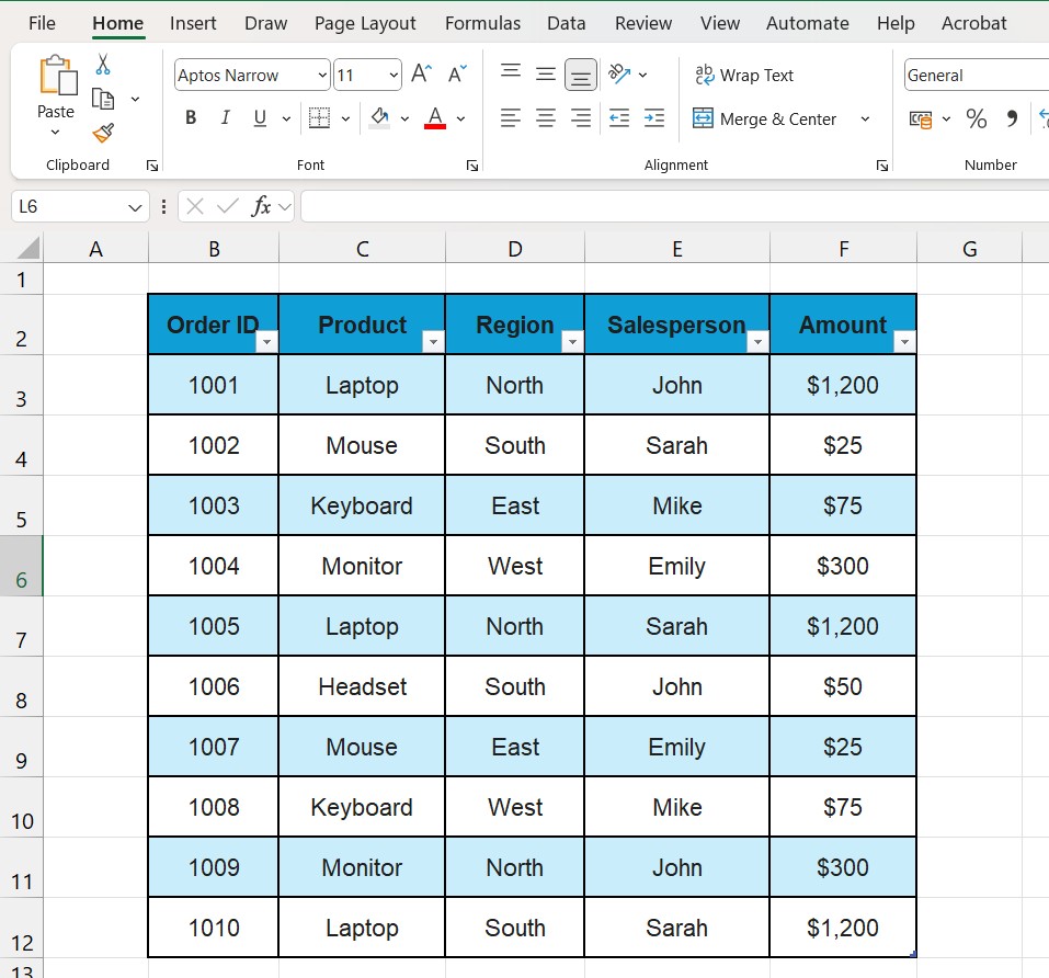
3. Click on Format as Table (in the Styles group).
4. Pick any color style you like (Blue, Green, Grey…).
5. A box will pop up asking “Where is the data for your table?”. Just click OK.

Boom! Your data now has alternating colors automatically.

• Bonus: If you add new rows later, the colors update automatically.

Method 2: Conditional Formatting (The Flexible Way)

Use this method if you don’t want to convert your data into an official Excel Table but still want the colors.

We will use a simple formula that checks if a row number is Even or Odd.

Step 1: Select Your Data Highlight the range of cells where you want the stripes (e.g., A2:E20). Do not include the header row.

Step 2: Open Conditional Formatting. Go to Home > Conditional Formatting > New Rule.

Step 3: Enter the Formula

1. Select the last option: “Use a formula to determine which cells to format”.
2. In the formula box, type exactly this: =MOD(ROW(),2)=0 (This formula tells Excel: “If the row number divided by 2 has no remainder (even number), color it.”)

Step 4: Pick a Color

1. Click the Format button.
2. Go to the Fill tab.
3. Choose a very light color (light grey or light blue work best).
4. Click OK twice.

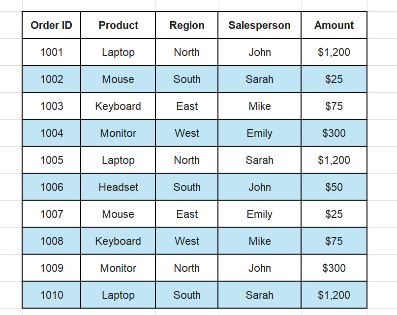
Now every even row (2, 4, 6…) will be colored, creating perfect zebra stripes.

Frequently Asked Questions (FAQ)

How do I remove the colors?

• If used Method 1 (Table): Click inside the table, go to the Table Design tab, and uncheck “Banded Rows”.
• If used Method 2 (Conditional): Select your data, go to Conditional Formatting > Clear Rules > Clear Rules from Selected Cells.

Can I color every 3rd row instead? Yes! In Method 2, change the formula to: =MOD(ROW(),3)=0.

Master the power of colors You just used a simple formula to color your rows, but did you know you can also color cells based on their value (like High/Low)?

👉 Learn more in our guide on How to Use Conditional Formatting in Excel.