
Looking for the Excel multiplication formula? You might be surprised to learn that there is no specific “MULTIPLY” function button. However, Excel offers powerful ways to perform calculations.
Unlike SUM or AVERAGE, there is no function named “MULTIPLY”.
However, Excel offers powerful ways to perform calculations. From the basic asterisk symbol to advanced techniques for updating thousands of prices at once, mastering the Excel multiplication formula is essential for any spreadsheet user.
Here are the 4 best methods to multiply in Excel, ranked from “Basic” to “Pro.”
Method 1: The Basic Asterisk (Standard Way)
The most common Excel multiplication formula uses the asterisk operator (*). This works exactly like a calculator.
How to do it:
- Click the cell where you want the result.
- Type
=to start the formula. - Select the first cell, type
*, and select the second cell. - Press Enter.
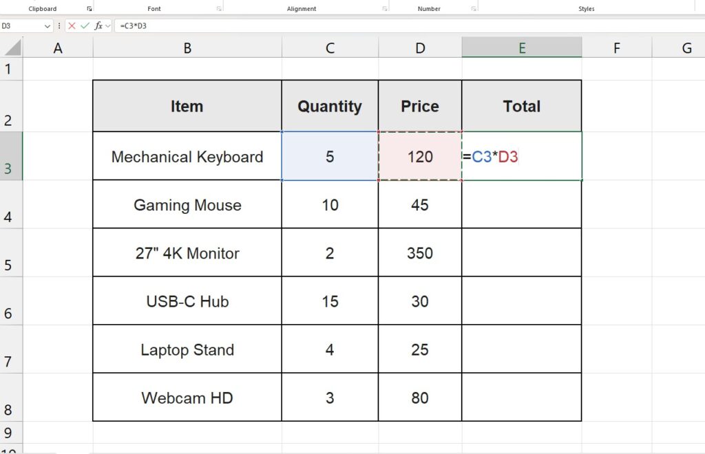
Example: To multiply Quantity (Column C) by Price (Column D), the formula is: =C3*D3
Note: You can multiply as many cells as you want, like =A1*B1*C1*10.
Method 2: The PRODUCT Function (Best for Ranges)
While the asterisk is great for two numbers, it gets messy if you need to multiply a list of 20 numbers. You don’t want to type =A1*A2*A3....
This is where the PRODUCT function shines. It multiplies all the numbers given as arguments and returns the product.
Formula Syntax: =PRODUCT(number1, [number2]...)
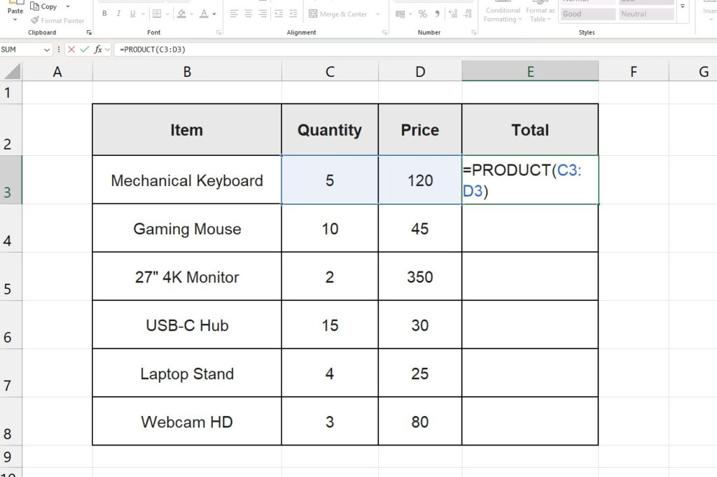
Real-world Example: If you want to multiply all values in the range A1 to A10: =PRODUCT(A1:A10)
This keeps your formula clean and easy to read.
Pro Tip: Working with long multiplication tables can be confusing if you scroll down and lose sight of your headers. To keep your ‘Price’ and ‘Quantity’ labels visible at all times, make sure to read our tutorial on How to Freeze the Top Row in Excel.
Method 3: Paste Special (The “Pro” Trick)
This is a hidden gem that many advanced users love.
Imagine you have a price list of 500 items, and you need to increase all prices by 10% (multiply by 1.10). You could create a helper column with a formula, but there is a faster way to change the values directly.
Step-by-Step:
- Type
1.10in any empty cell and copy it (Ctrl + C). - Select the range of prices you want to update.
- Right-click and choose Paste Special… (or press
Ctrl + Alt + V). - In the “Operation” section, select Multiply.
- Click OK.
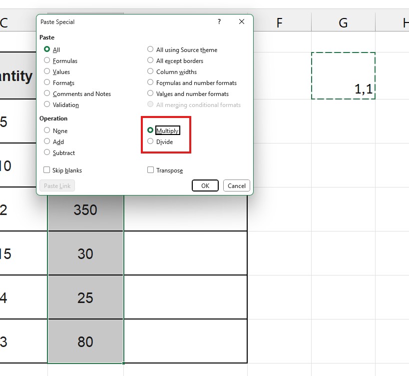
Boom. Excel instantly multiplies every selected cell by 1.10. You can now delete the helper cell. No formulas required!
Method 4: Multiplying Entire Columns (Dynamic Arrays)
If you are using Excel 365 or Excel 2021, you can use Dynamic Arrays to create a multiplication table that spills automatically.
Instead of writing a formula in row 2 and dragging it down, you can multiply whole array ranges.
The Formula: =B2:B10 * C2:C10
When you press Enter, Excel understands you want to multiply the corresponding rows and fills the results down instantly. If you see a Spill Error, make sure the cells below are empty.
(See our guide on how to fix Spill Errors for more details)
Troubleshooting: Why do I get a #VALUE! Error?
If your Excel multiplication formula returns a #VALUE! error, it usually means one of the cells contains text instead of a number.
- Check for Spaces: sometimes a number like ” 100″ has a leading space, making Excel treat it as text.
- Check formatting: Ensure your cells are formatted as “General” or “Number,” not “Text.”
Conclusion
While there is no button labeled “Multiply,” the flexibility of the Excel multiplication formula gives you total control.
- Use the Asterisk (
*) for quick, simple math. - Use PRODUCT for long lists of numbers.
- Use Paste Special > Multiply to bulk-update data without formulas.
Mastering these basics is the first step to building professional financial dashboards and inventory reports.
Once you have calculated all your totals using these formulas, you might want to summarize the data to see the big picture. Check out our guide on How to Create a Pivot Table in Excel to analyze your sales figures instantly without adding more complex formulas.