How to Create a Drop-Down List in Excel (Step-by-Step Guide)

Do you want to stop people from making typing mistakes in your spreadsheet? Or maybe you just want to make data entry faster?

The solution is a Drop-Down List.

Instead of typing “Yes”, “No”, or “Maybe” manually (and risking typos like “Yess”), a drop-down list lets users select from a predefined menu. It makes your Excel sheets look professional, clean, and error-free.

In this guide, you will learn the fastest way to create a drop-down list in Excel using Data Validation.

Why Use Drop-Down Lists?

• Consistency: Ensures everyone enters data exactly the same way.
• Speed: Selecting from a list is faster than typing.
• Professionalism: It turns a basic sheet into an interactive form.

Method 1: The Quick Manual List (For small options)

If you only have a few options (like Yes/No or High/Medium/Low), this is the fastest method.

Step 1: Select the Cell Click on the cell (or range of cells) where you want the list to appear.

Step 2: Go to Data Validation

1. Go to the Data tab on the top ribbon.
2. Look for the “Data Tools” group and click Data Validation.

Step 3: Configure the Settings A pop-up window will appear.

• Under Allow, select List.
• In the Source box, type your options separated by a comma.
  • Example: Yes,No,Maybe

• Click OK.

Now, when you click that cell, a small arrow will appear, letting you choose from your list.

Method 2: Creating a List from a Range (The Pro Way)

If you have a long list of items (like 50 employee names or product codes), typing them manually with commas is a nightmare. Instead, store them in a spreadsheet.

Step 1: Create Your Source List Go to a separate sheet (or the side of your current sheet) and type your list in a column.

• Tip: Give this list a header, like “Departments”.

Step 2: Start Data Validation Select the cell where you want the drop-down menu and go back to Data > Data Validation.

Step 3: Select the Source

• Under Allow, choose List.
• Click inside the Source box.
• Instead of typing text, use your mouse to highlight the cells containing your list (e.g., =Sheet2!$A$2:$A$10).

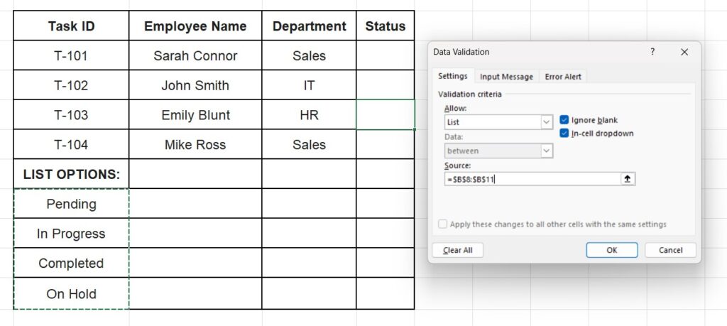
• Click OK.

Why is this better? If you need to change an option later (e.g., change “Marketing” to “Growth”), you just update the source cell, and the drop-down list updates automatically.

How to Remove a Drop-Down List

Did you make a mistake or just want to go back to normal cells?

1. Select the cell(s) with the drop-down list.
2. Go to Data > Data Validation.
3. Click the Clear All button in the bottom left corner.
4. Click OK.

Frequently Asked Questions (FAQ)

Can I add color to my drop-down list? The list itself is standard gray/white, but you can make the cell change color based on the selection using Conditional Formatting. For example, turn the cell Green if “Yes” is selected and Red if “No” is selected.

How do I copy the drop-down list to other cells? Just copy the cell (Ctrl + C) and paste it (Ctrl + V) wherever you want. You can also drag the fill handle (the small square in the corner) down to apply it to a whole column.